Statistical Modeling and Objective function
Through forecasting projects, I’ve learned a crucial lesson that’s often overlooked in introductory courses: your model is only as good as its loss function, and the default choice is often the wrong one.
We all start by learning to use Mean Squared Error (MSE) for our regression tasks. It’s simple, intuitive, and the default in most libraries. But blindly applying it to every problem is like trying to use a hammer for every job in a toolbox. For many real-world industrial cases, it’s a critical mistake. Let’s explore why.
The Default: MSE and its Hidden Assumption
When you train a Gradient Boosting model (or almost any regression model) using Mean Squared Error (MSE) as the loss function, you’re doing more than just penalizing large errors. You are implicitly making a powerful statistical assumption: that the errors of your model will follow a Normal (or Gaussian) distribution.

Symmetrical, continuous, and defined for all real numbers. MSE assumes residuals follow this shape.
This assumption works perfectly fine for certain problems. In the work with energy demand forecasting, the target variable (megawatt-hours) is continuous and typically high-volume. The demand curve is smooth, and the errors tend to cluster symmetrically around zero. In this scenario, the Normal distribution is a reasonable approximation of reality, and MSE is an excellent choice. It aggressively penalizes large deviations, pushing the model to be accurate for this high-stakes task.
But what happens when the data doesn’t look like a nice, continuous bell curve?
When the Default Fails: The World of Count Data
Now, let’s consider projects on inventory demand and strawberry yield forecasting. Here, the target variable is fundamentally different:
- You can’t sell 2.43 spare parts.
- A farmer counts 5 ripe strawberries, not 5.7.
This is count data. It’s discrete, non-negative, and often full of zeros. This is especially true for intermittent demand in inventory management, where a specific part might not be sold for days or weeks, followed by a sudden sale.
If you use MSE on this type of data, you’re asking your model to play by the wrong rules. The model might predict negative sales (-0.5 units) or fractional demand (1.25 units), which is nonsensical in the real world. This mismatch between the model’s assumption (Normal distribution) and the data’s reality (a discrete count process) leads to poor performance and unreliable forecasts.
However, here’s a catch: pragmatically, MSE works quite well if the dataset is continuous (not intermittent).
The Right Tools for the Job: Poisson & Negative Binomial
To correctly model count data, we need loss functions derived from distributions designed for counts. This is where the Poisson and Negative Binomial distributions come in.
Poisson: The Go-To for Simple Counts
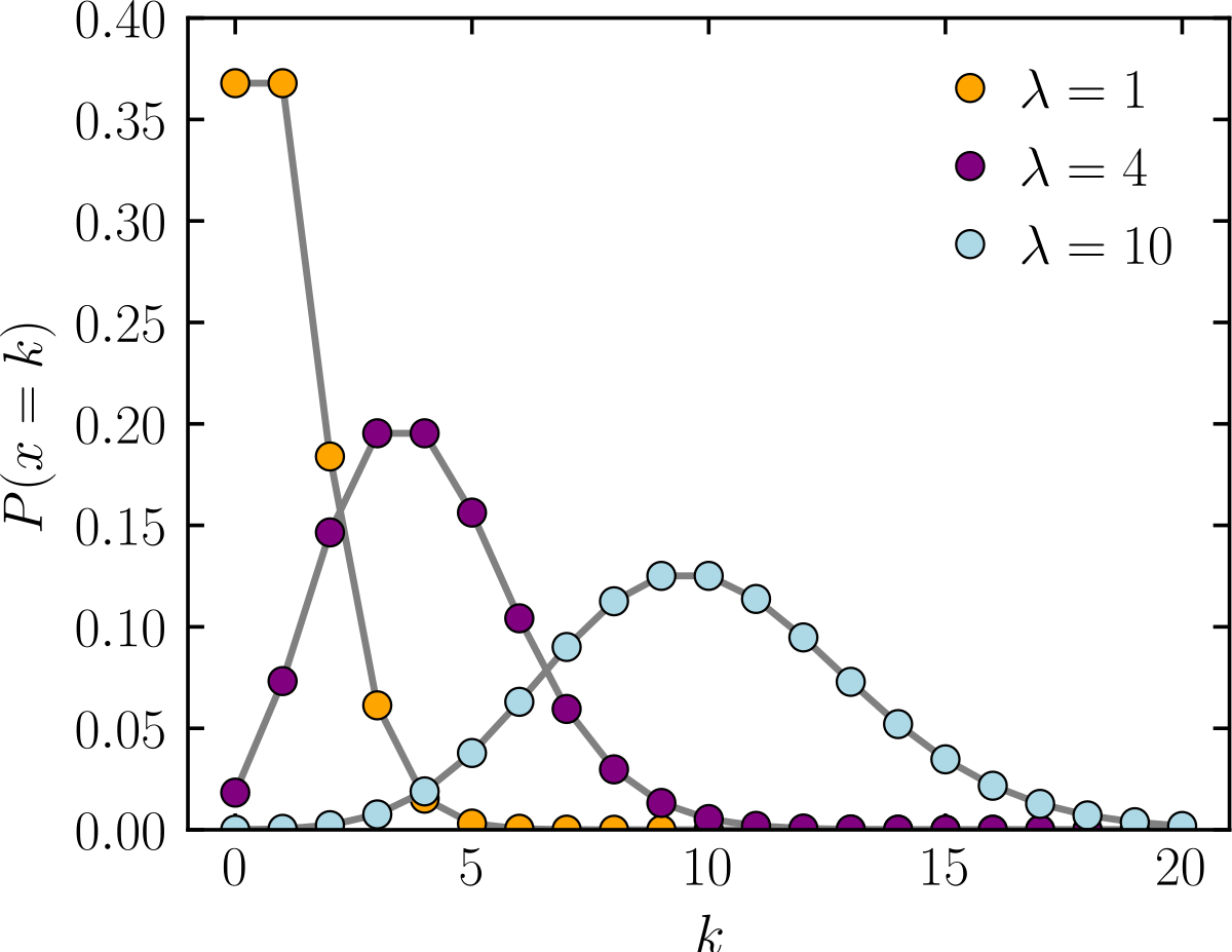
The Poisson distribution models the probability of a number of events happening in a fixed interval. It’s perfect for data that consists of non-negative integer counts.

Discrete, non-negative, and defined only for integers. The “spikey” nature matches real-world counts.
By setting the objective function in my GBDT to poisson, I’m no longer just predicting a value; I’m telling the model to predict the rate (\(\lambda\)) of an event. I’m aligning the model’s objective with the data’s true nature. This immediately prevents predictions of negative values and grounds the model in the reality of a counting process.
Negative Binomial: For Messy, Real-World Counts
The Poisson distribution has one strict limitation: it assumes the mean and the variance of the data are equal. In my experience, real-world data is rarely this well-behaved.
Take inventory demand, for example. The average demand for a part might be 0.2 units per day, but when a sale occurs, it could be for 5 units. This “lumpy” demand is highly variable. This phenomenon, where the variance is much larger than the mean, is called over-dispersion.
This is where the Negative Binomial distribution shines. It’s a count data distribution like Poisson, but it has an extra parameter that allows the variance to be greater than the mean.

Handles over-dispersion gracefully—note the heavier tail compared to Poisson.
Using a Negative Binomial loss function (or a tweedie objective in many libraries) gives the model the flexibility to handle this spiky, over-dispersed data, leading to far more accurate and stable forecasts for lumpy demand patterns.
The Connection Between Objective Functions and Statistical Modeling via MLE
At the heart of every machine learning loss function lies a statistical distribution assumption. This connection is formalized through Maximum Likelihood Estimation (MLE), a fundamental principle that bridges probability theory and optimization.
1. The Principle of Maximum Likelihood Estimation (MLE)
MLE answers the question: “Given observed data, what model parameters make this data most probable?”
- Likelihood Function: For a dataset \(\{y_i\}_{i=1}^n\) and predictions \(\{\hat{y}_i\}_{i=1}^n\), the likelihood under a distribution \(P\) is:
\(L(\theta) = \prod_{i=1}^n P(y_i | \theta, \hat{y}_i)\) - Log-Likelihood: Converting products to sums for numerical stability:
\(\log L(\theta) = \sum_{i=1}^n \log P(y_i | \theta, \hat{y}_i)\) - Negative Log-Likelihood (NLL): Flipped to a minimization problem:
\(\text{NLL}(\theta) = -\sum_{i=1}^n \log P(y_i | \theta, \hat{y}_i)\)
This NLL becomes the loss function we minimize during training.
2. From Distributions to Loss Functions
The choice of distribution \(P\) directly determines the loss function:
| Distribution | Loss Function | Use Case |
|---|---|---|
| Normal (Gaussian) | MSE | Continuous, symmetric errors |
| Poisson | Poisson loss | Simple counts (mean ≈ variance) |
| Negative Binomial | NBinom/Tweedie loss | Over-dispersed counts |
3. Why Does This Matter?
- Correctness: Using MSE for count data violates the Normal assumption, leading to biased predictions (e.g., negative counts).
- Efficiency: The right loss function (derived from the true data distribution) leads to faster convergence.
- Interpretability: A Poisson/Negative Binomial loss directly models count rates, aligning with business logic (e.g., “units sold per day”).
Key Takeaway
Your loss function is a distributional assumption in disguise. Choose it based on the data’s statistical nature, not convenience. MLE provides the mathematical framework to derive the right loss function for your problem.
